Iris Dataset
In the 1820s, a botanist named Edgar Anderson collected morphologic variation data on three related species of irises. In 1936, statistician and biologist Ronald Fisher would use this data to introduce a model called linear discriminant analysis, which he used to desribe how the iris species could be correctly classified based on their measured features.
Iris Dataset
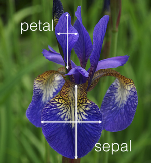
- 150 Samples of 4 different measurements (sepal length, sepal width, petal length, petal width)
- 50 Samples each of different iris species (setosa, versicolor, and virginica)
In [94]:
import seaborn
import matplotlib
import matplotlib.pyplot as pyplot
import pandas
%matplotlib inline
seaborn.set(style="white", color_codes=True)
# import load_iris function from datasets module
from sklearn.datasets import load_iris
Import Data
In [95]:
# save "bunch" object containing iris dataset and its attributes
iris = load_iris()
type(iris)
Out[95]:
In [96]:
# print the iris data
print(iris.data)
In [97]:
# print the names of the four features
print(iris.feature_names)
In [98]:
# print integers representing the species of each observation
print(iris.target)
In [99]:
# print the encoding scheme for species: 0 = setosa, 1 = versicolor, 2 = virginica
print(iris.target_names)
In [100]:
# check the types of the features and response
print(type(iris.data))
print(type(iris.target))
In [101]:
# check the shape of the features (first dimension = number of observations, second dimensions = number of features)
print(iris.data.shape)
In [102]:
# check the shape of the response (single dimension matching the number of observations)
print(iris.target.shape)
In [103]:
# store feature matrix in "X"
X = iris.data

# store response vector in "y"
y = iris.target
Convert to dataframe
In [104]:
# Create a dataframe from iris data (useful for plotting)
iris_structure = { iris.feature_names[0]: iris.data[:,0], iris.feature_names[1]: iris.data[:,1], \
                  iris.feature_names[2]: iris.data[:,2], iris.feature_names[3]: iris.data[:,3], \
                  'Species': iris.target_names[iris.target]}
iris_df = pandas.DataFrame( iris_structure );
iris_df
Out[104]:
Exploratory Data Analysis
In [105]:
# One piece of information missing in the plots above is what species each plant is
# We'll use seaborn's FacetGrid to color the scatterplot by species
seaborn.FacetGrid(iris_df, hue="Species", size=5) \
   .map(pyplot.scatter, "sepal length (cm)", "sepal width (cm)") \
   .add_legend()
Out[105]:

In [106]:
iris.target_names
Out[106]:
In [107]:
seaborn.pairplot( iris_df, hue="Species", size=3, diag_kind="kde")
Out[107]:

From the data visualization, the setosa species looks linearly separable from versicolor and virginica. However, versicolor and virginica do not appear to be linearly separable.
Models and Model Comparison
In [108]:
from sklearn import model_selection
from sklearn.model_selection import RepeatedKFold
from sklearn.linear_model import LogisticRegression
from sklearn.tree import DecisionTreeClassifier
from sklearn.neighbors import KNeighborsClassifier
from sklearn.discriminant_analysis import LinearDiscriminantAnalysis, QuadraticDiscriminantAnalysis
from sklearn.naive_bayes import GaussianNB
from sklearn.ensemble import RandomForestClassifier, AdaBoostClassifier
from sklearn.svm import SVC
from sklearn.gaussian_process import GaussianProcessClassifier
from sklearn.gaussian_process.kernels import RBF
from sklearn.neural_network import MLPClassifier
In [114]:
# prepare configuration for cross validation test harness
seed = 1
# prepare models
models = []
models.append(('LR',    'Logistic Regression', LogisticRegression()))
models.append(('LDA',   'Linear Discriminant Analysis', LinearDiscriminantAnalysis()))
models.append(('QDA',   'Quadratic Discriminant Analysis', QuadraticDiscriminantAnalysis()))
models.append(('KNN1',  'K-Nearest Neighbors (K=1)', KNeighborsClassifier(n_neighbors=1)))
models.append(('KNN3',  'K-Nearest Neighbors (K=3)', KNeighborsClassifier(n_neighbors=3)))
models.append(('KNN5',  'K-Nearest Neighbors (K=5)', KNeighborsClassifier(n_neighbors=5)))
models.append(('GP',    'Gaussian Process Classifier', GaussianProcessClassifier()))
models.append(('CART',  'Decision Tree Classifier', DecisionTreeClassifier()))
models.append(('RF',    'Random Forest', RandomForestClassifier(n_estimators=10, max_features=2)))
models.append(('GB',    'AdaBoost Gradient Boosting', AdaBoostClassifier()))
models.append(('NB',    'Naive Bayes', GaussianNB()))
models.append(('SVM_L', 'Support Vector Machine (Linear Kernel)', SVC(kernel='linear')))
models.append(('SVM_R', 'Support Vector Machine (Radial Kernel)', SVC(gamma=2,C=1)))
models.append(('NN',    'Multilayer Perceptron', MLPClassifier(alpha=1,learning_rate_init=0.01)))
# evaluate each model in turn
results = []
names = []
scoring = 'accuracy'
print( "%40s  %8s (%8s)" % ("Model", "Accuracy", "Std Dev") );
for shortname, longname, model in models:
	kfold = model_selection.RepeatedKFold(n_splits=10, n_repeats=3, random_state=seed)
	cv_results = model_selection.cross_val_score(model, X, y, cv=kfold, scoring=scoring)
	results.append(cv_results)
	names.append(shortname)
	msg = "%40s: %f (%f)" % (longname, cv_results.mean(), cv_results.std())
	print(msg)
# boxplot algorithm comparison
font = {'family' : 'DejaVu Sans',
        'weight' : 'bold',
        'size'   : 22}
matplotlib.rc('font', **font)
fig = pyplot.figure(figsize=(12,10))
fig.suptitle('Model Accuracy (10-fold cross-validation)')
ax = fig.add_subplot(111)
pyplot.boxplot(results)
ax.set_xticklabels(names)
pyplot.show()

Perhaps not surprisingly, the LDA model performed the best (lower error bounds than the other models and more interpretable than the Neural Network model).