The Problem Statement
The MNIST dataset is a now classic dataset of handwritten digits from 0-9 available at http://yann.lecun.com/exdb/mnist/. Included in the dataset are 60,000 annotated training examples and a test set of 10,000 examples. Each digit has been captured electronically as a 28x28x1 bit map, where the greyscale value (0-255) of each pixel is encoded for each of the 28x28 = 784 locations. This means that there are 784^256 distinct image possibilities - which is not a trivial challenge.
The goal is to use the training data to create a model that will accurately predict the classification of the handwritten digits in the test set. Researchers have used a variety of methods for over 20 years, the latest and best results coming from Convolutional Neural Networks (CNNs). As I started this project, my main goal was to achieve a good accuracy on the test set. I looked over several other approaches and tried to reproduce the results. The training took a long time! Then I tried a few things to increase the accuracy and I waited. And waited. And waited some more. As I continued to work and try new convnets, I realized a new goal: to have my convnet train in a reasonable time. For me, this is about 12 hours maximum (somewhere around an overnight time period). If you're lucky enough to have a good NVIDIA GPU, you can use this to your advantage by using Tensorflow-GPU and try some higher parameter models. But if you're limited to a CPU, you're likely going to be similarly constrained.
import pandas as pd
import numpy as np
import matplotlib.pyplot as plt
import seaborn as sns
import random
import cv2

%matplotlib inline

np.random.seed(42)

from pylab import gcf

from scipy.misc import imresize
from skimage.transform import resize
from sklearn.model_selection import train_test_split
from sklearn.metrics import confusion_matrix

from keras.utils.np_utils import to_categorical
from keras.models import Sequential
from keras.layers import Dense, Dropout, Flatten, Conv2D, MaxPool2D, SpatialDropout2D
from keras.optimizers import Adam
from keras.preprocessing.image import ImageDataGenerator

sns.set(style='white', context='notebook', palette='deep')
Exploratory Data Analysis
Kaggle provides the test and train datasets in .csv format. There are 60,000 train records and 10,000 test records.
trainRows = pd.read_csv("../input/train.csv")
testRows = pd.read_csv("../input/test.csv")
Each record in the train dataset has 28x28 + 1 = 785 columns: Column '1' is the record label - the curated class of this handwritten digit (i.e., a number between 0-9) and 784 columns for pixel intensities.
# train dimensions
trainRows.shape
# test dimensions
testRows.shape
trainRows.head()
The test dataset is much like the train dataset except for the missing 'label' column. This is the value we are to predict.
testRows.head()
# split train into trainX and trainY (label)
trainY = trainRows["label"]
# by removing the label from trainX, dataset is same as test
trainX = trainRows.drop(labels=["label"],axis=1)
trainXRows = trainX
Reshape test and train vectors into bitmaps
# these are 28x28 captures
trainX = trainX.values.reshape(-1,28,28,1)
test = testRows.values.reshape(-1,28,28,1)
# greyscale values are encoded 2**8 = 0-255 different values.  Scale to 0-1 range:
trainX = trainX / 255.0
trainXRows = trainXRows / 255.0
test = test / 255.0
Check counts of each training digit
trainY.value_counts().plot(kind='bar')
trainY.value_counts()

Visualizing the "average" handwritten digit
If each curated handwritten digit is overlayed on each other for each class, it is possible to create an average intensity at each pixel for that digit and create an average digit image. This is done below and suggests that simply making filters out of these and convolving with test data could produce a fairly accurate model.
import matplotlib

cmap = matplotlib.cm.get_cmap('Spectral')
fig = plt.figure(figsize=(16,16))
# i'm sure there's a much more "pythonic" way to do this. ¯\_(ツ)_/¯
for i in range(10):
    idxDigit = [j for j in range(len(trainX)) if trainY[j] == i]  # group by label
    meanPixels = trainXRows.iloc[idxDigit].mean()  # take mean of all '7s', for instance
    digitMeans = meanPixels.values.reshape(-1,28,28,1)
    plt.subplot(4,3,i+1)
    plt.imshow(digitMeans[0][:,:,0],cmap=cmap)
    plt.colorbar()

plt.show()

Average Digit
In the same way, it is possible to create an overall average digit, shown below. Also shown is the distribution of intensity values.
import matplotlib
cmap = matplotlib.cm.get_cmap('Spectral')
fig = plt.figure(figsize=(10,10))
digitMeans = trainXRows.mean().values.reshape(-1,28,28,1)
plt.imshow(digitMeans[0][:,:,0],cmap=cmap)
plt.colorbar()
plt.show()

# next, take a look at the intensity values to see if we can apply parametric significance tests for individual pixels
fig = plt.figure(figsize=(16,8))
plt.subplot(1,2,1)
plt.hist(trainXRows.mean(),30)
# on the right hand side, omit first peak of zeros so get a better look at distribution
plt.subplot(1,2,2)
plt.hist(trainXRows.mean(),30)
plt.axis([0.01,0.6,0,50])


Which pixels are important for each digit?
The individual pixel means and standard deviations for each digit can be contrasted with the overall digit heatmap. To do this, we compare the class pixel means and standard deviations with the non-class pixel means and standard deviations. The intensity data are not normally distributed so parametric signficance tests are not applicable here. Nevertheless, we press on! This plot of z-scores should give some indication of which pixels are important for each digit (blue indicates postive z-score, red indicates negative). So, for instance, the red circular region in the '0' digit shown below is an area where pixels are not expected to have high intensity for the number 0. The blue regions, however, are associated with the '0' digit over the background non-zero digits.
import matplotlib
import math
cmap = matplotlib.cm.get_cmap('Spectral')
fig = plt.figure(figsize=(16,16))
for i in range(10):
    idxDigit = [j for j in range(len(trainX)) if trainY[j] == i]  # group by label
    idxNonDigit = set( range(len(trainX)) ) - set( idxDigit )
    idxNonDigit = list( idxNonDigit )
    meanDigitPixels = trainXRows.iloc[idxDigit].mean()  # take mean of all '7s', for instance
    stdDigitPixels = trainXRows.iloc[idxDigit].std()
    numDigit = len(idxDigit)
    numNonDigit = len(idxNonDigit)
    meanNonDigitPixels = trainXRows.iloc[idxNonDigit].mean()
    stdNonDigitPixels = trainXRows.iloc[idxNonDigit].std()
    pooledVariance = (stdDigitPixels**2)/numDigit + (stdNonDigitPixels**2)/numNonDigit
    zscores = ( meanDigitPixels - meanNonDigitPixels ) / pooledVariance.apply(np.sqrt)
    zImage = zscores.values.reshape(-1,28,28,1)
    plt.subplot(4,3,i+1)
    plt.imshow(zImage[0][:,:,0],cmap=cmap)
    plt.colorbar()

plt.show()

Create validation set
From the training set trainX, we create a validation set using 10% (0.1) of the 42000 training records. This will allow us to evaluate model performance and tune hyperparameters without having to test on our 'true' test set.
random_seed = 1984
trainY = to_categorical( trainY, num_classes = 10 )
subTrainX, valX, subTrainY, valY = train_test_split(trainX, trainY, test_size = 0.1, random_state=random_seed)
CNN
The best and most recent results for this problem have come from convolutional neural networks. So, that's the approach here - let the CNN do the heavy lifting to find the which sets of features best predict a given digit. The Keras Sequential API makes constructing CNN layers easy and intuitive. What's NOT immediately intuitive is how exactly to construct the network. To do this, it's best to start with a similar architecture to successful CNNs from the ImageNet competition. The first convnet to break onto the scene in the ImageNet competition and do well was AlexNet in 2012. The architecture for this CNN is as follows:
Convolution2D - 96 11x11 filters at stride 4
Max Pooling 3x3, stride 2
Normalization
Convolution 2D - 256 5x5 filters at stride 1
Max Pooling 3x3
Normalization
Convolution 2D - 384 3x3 filters at stride 1
Convolution 2D - 384 3x3 filters at stride 1
Convolution 2D - 256 3x3 filters at stride 1
Dense layer, 4096 neurons
Dense layer, 4096 neurons
Output Dense layer, 1000 neurons (final scores for each image class)
Each of the successive winners of ImageNet were CNNs and each retained some similar architecture to the original AlexNet in the approach of applying successive convolutions, followed by pooling (and reducing/eliminating the dense layers at the end).
About the Layers
- 2D Convolution This layer convolves a filter of size (kernel_size) with the input layer. Smaller filters seem to be what most of the ImageNet CNN's use (3x3 or 5x5). Intuitively, this makes some sense since a 3x3 filter convolved with the input image would do a better job retaining local features than a larger filter, which would average out some of the finer detail. What's not clear initially...what are the filters? Also not clear - how many filters to use. I found this post describing the initial filters: https://datascience.stackexchange.com/questions/16463/what-is-are-the-default-filters-used-by-keras-convolution2d So, the initial filters are random drawn from the range (-6/(num_in+num_out), 6/(num_in+num_out)) and are updated accordingly through backpropagation. As far as how many filters to use...there doesn't seem to be a guide but intuitively, I'd consider the size of the filter to be somewhat related. After all, there are just so many 3x3 filters that you can have before you start to see two or more filters that are quite similar. I'd think that'd this would be something akin to having some colinear nodes in your network. So, I'm inclined to use a small number of filters when using 3x3 kernels, and increase the number when using larger kernels.
- Dropout Sets a proportion of inputs to zero at each update, effectively shutting down certain flows through the network, forcing the network to learn through a different route. This helps prevent overfitting and make a more robust network. It's not clear what to set this proportion to at each point but intuitively, it seems that if you set the Dropout too high, you're going to get a more "average" network since you're essentially forcing all the different paths to more or less look the same. Conversely, if you set it too low or omit it altogether, you're more likely to overfit the training data as it would allow niche paths through the network that only fire for a small part of the training data.
- Pooling Pooling downsamples the data. So, for instance a 2x2 pooling filter considers the data over a 2x2 region for each output pixel. The effect of a 2x2 filter (with implicit stride 2) on an input set is that the dimensions are halved. MaxPooling is pooling that outputs the maximum activation over each region evaluated. Now, if you saw some of the input MNIST data, you probably couldn't help but notice that they're already pretty well downsampled. Going from a handwritten digit to a 28x28 map results in some significant pixelation. When I first approached this problem, I thought I'd skip the downsampling since the data couldn't possibly survive more downsampling, right? So much for that intuition. Perhaps that would be true if I had a good GPU, but while downsampling is of course lossy, it also has a few benefits. One is that it can retain much of the same information about feature hits for only a comparatively small loss of information. The other, and most important benefit is that it cuts down on the number of parameters to compute in the network and the fewer the parameters, the faster the training time.
- Flattening Simply reshapes inputs into a 1D output vector.
- Dense Basic fully-connected layer between input and output where output = activation(dot(input,kernel) + bias). Argument to this specifies how many nodes are in the layer.
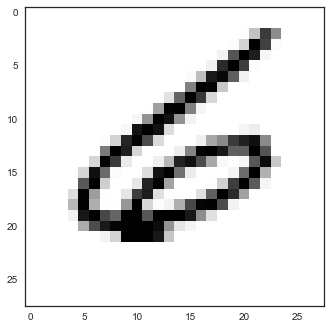
Model Architecture
Most ImageNet CNNs have the same general architecture - two successive convolutions with smallish filters and the nonlinear ReLu activation function, followed by a pooling step. I followed the same idea here. For the first convolution layer, I chose "valid" as the padding. This effectively trims out the outermost layer of pixels from the image, turning a 28x28 image into a 26x26 convolution with the first set of filters. I chose "valid" because it looked like the information in that outer layer wasn't worth keeping (mostly all zeros - see the picture of the training set '6' digit at the top of this notebook, for example). If these were ImageNet pictures, with picture details extending all the way to the boundaries, then I'd want to use "same" at this first convolution step. The next convolution step is also 32 3x3 filters followed by pooling. The pooling step reduces the dimensions of the convolved images to 13x13. Finally, a dropout layer is applied, which keeps the network robust. The same block structure is then repeated, resulting in a 6x6 layer of convolved images. Some newer ImageNet networks have eliminated the fully connected layers altogether, but when I made mine smaller from 128 nodes, I got poorer results.
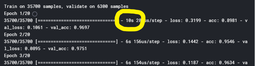
Suggestions for your model architecture: Firstly, try to reproduce the results from some Kaggle kernels. Pay close attention to the time taken per epoch and see if you get roughly comparable performance:
If you don't then you will have to modify your approach by shrinking your filters, shrinking your number of filters, decreasing the number of fully connected nodes, decreasing the number of layers, and/or pooling more to reduce the dimensionality. Once you have figured out what kind of performance you can expect from your machine, then you can start experimenting with data augmentation, more filters, larger filters, etc.
Hyperparameters
In addition to the general model architecture, there are a slew of dials to adjust. And of course, adjusting one knob usually requires appropriately adjusting one or more of the other knobs.
- number of filters (filters) in each convolution step - Too few and your network won't have the complexity to separate close cases. Too many and your network will take a long time to train, might overfit, and will be difficult to optimize since there will likely be a complex loss landscape. I had to stick with low numbers for my network since every trained so slow. Why '32' and not '30' or '40'? No reason, other than a vestigial preference for powers of 2 from the old days of computer science.
- filter size (kernel_size) - Newer convnets are moving towards smaller filters and since the complexity and training time depend on the filter size, networks will smaller filters take less time to train (all other things being equal). You can stack smaller filters and gain the same receptive field as a larger filter and still have a network of less complexity than just using a larger filter. I chose 3x3 filters because my computer is a dinosaur sinking in a tar pit.
- pooling type and size - On the surface, it's hard to justify pooling. Why in the world should we have to downsample an already pixelated bunch of tiny 28x28 images. Then, I ran my first convnet and it never even finished one epoch. But it's easy to see the benefits - you can still retain much information about feature hits and only seemingly incur a smallish loss of sensitivity while enjoying a network of lower complexity (and faster training time). For this MNIST problem, you probably don't want to go any higher than 2x2 since the images are already so small. But for larger images, pooling and adjusting the stride can drop the complexity and allow for deeper networks.
- dense layer node count - Again, some of the latest networks in ImageNet have removed the dense layers altogether (AlexNet had 3 dense layers at the end). The dense layers can add a LOT of complexity to your model. When trying different node counts, be sure to use the model.summary() feature to see how much time you'd be devoting to that last dense layer. I tried to drop the number on this layer to 32 or 16 and the network didn't train at all. I did no optimizations of the '128' number - I just chose it because it was large but not too large and had that nice, comforting power of 2 feel about it. And someone else used it before me, so it has to be well thought out, right?
- dropout rate - Yeah, this is another magic number. See dropout discussion above in the layers section. I did no optimizations, simply picked 0.25. But since it's a power of 2, (2^(-2)), it's probably correct.
- batch size - Ideally, we'd run all the training data through the network, calculate the gradient, move in the right direction with just the perfect step size and quickly get to the bottom of our loss landscape, then sit back and enjoy all the accompanying wealth and fame for creating such an awesome convnet. If we tried this our gradient estimate would be perfect every time but it takes a LOT of memory and a long time to process all of the data just to take one step. And there's lots of steps. So, what if we tried the complete opposite approach and just considered each one of the 42000 training examples one at a time, calculated the gradient, and then stepped in the direction of the largest negative gradient? If we did that, the path would look more like a drunken hiker meandering along the way to the bottom, sometimes taking missteps and going in the wrong direction (of the overall gradient). So, what's the solution? Considering not one, but many (but not too many!) examples - and this is the batch size. What you really want here is enough training examples to form a good representation of the true gradient. I chose 128 because it's a power of 2 and therefore has to be correct. But really, I chose 128 because I wanted to try to ensure that each of the 10 digits likely had some representation in the gradient calculation. An alternative way would be to decrease the batch size and make a stratified sample of each of the digits - say 3-4 from each digit class and have a batch size of 30-40 that way, each gradient calculation would have input from each digit and still be smallish. Another feature that would be nice to have would be a way to adaptively increase the batch size when the gradient started getting smaller as this would possibly indicate that you're reaching a minimum and therefore would want to ensure that each step is in the right direction.
- epochs - One epoch represents one pass of the whole training set through the model. The number of epochs needed is going to vary from case to case. If the training set is large enough, the whole optimization might just about converge before one epoch. In general, you want to see the loss or accuracy level off (see model evaluation below), note the number of epochs taken, then set that as your number of epochs.
- optimizer and learning rate - There are at least 8 different optimizers to choose from in Keras. I went with Adam. Adam has nice properties and a history of good results but Nadam might be an even better choice, IMO, because the method of computing momentum seems more correct. With Adam, I went with the default learning rate of 0.001 because it seemed to work well.
model = Sequential()

model.add(Conv2D(filters = 32, kernel_size = (3,3), padding = 'valid',
                 activation ='relu', input_shape = (28,28,1)))
model.add(Conv2D(filters = 32, kernel_size = (3,3), padding = 'same',
                 activation ='relu'))
model.add(MaxPool2D(pool_size=(2,2)))
model.add(SpatialDropout2D(0.25))


model.add(Conv2D(filters = 32, kernel_size = (3,3), padding = 'same',
                 activation ='relu'))
model.add(Conv2D(filters = 32, kernel_size = (3,3), padding = 'same',
                 activation ='relu'))
model.add(MaxPool2D(pool_size=(2,2)))
model.add(SpatialDropout2D(0.25))


model.add(Flatten())
model.add(Dense(128, activation = "relu"))
model.add(Dropout(0.5))
model.add(Dense(10, activation = "softmax"))

model.compile(optimizer = Adam(), loss = "categorical_crossentropy", metrics=["accuracy"])
model.summary()
epochs = 10
batch_size = 128
Data augmentation
Keras provides another very useful proprocessing tool to increase the training set size: ImageDataGenerator. ImageDataGenerator takes input images and performs random permutations on them to create a new set of training images. For instance, you can specify a random rotation of a range of degrees, random zooming in/out of a specified scaling, cropping, shear, shift, and flips. This tool should be used when there are a limited amount of training samples or if a higher accuracy is paramount and you have the compute power to use it.
imageDataGenerator = ImageDataGenerator(
        featurewise_center=False,  # set input mean to 0 over the dataset
        samplewise_center=False,  # set each sample mean to 0
        featurewise_std_normalization=False,  # divide inputs by std of the dataset
        samplewise_std_normalization=False,  # divide each input by its std
        zca_whitening=False,  # apply ZCA whitening
        rotation_range=10,  # randomly rotate images in the range (degrees, 0 to 180)
        zoom_range = 0.1, # Randomly zoom image
        width_shift_range=0.1,  # randomly shift images horizontally (fraction of total width)
        height_shift_range=0.1,  # randomly shift images vertically (fraction of total height)
        horizontal_flip=False,  # randomly flip images
        vertical_flip=False)  # randomly flip images

imageDataGenerator.fit(subTrainX)
# Uncomment this line if you have the GPU to train this network with augmented data

#fit = model.fit_generator(datagen.flow(subTrainX,subTrainY, batch_size=32), epochs = epochs, validation_data = (valX,valY), verbose = 2, steps_per_epoch=subTrainX.shape[0]/32 )

#otherwise, use this fit
fit = model.fit(subTrainX, subTrainY, batch_size = batch_size, epochs = epochs, verbose = 2, validation_data = (valX,valY)  )
Model Evaluation
The first thing that sticks out when looking at the training and validation curves is that the validation accuracy is higher than the training accuracy (and validation loss is less than the training loss). How can this be? It is because of the dropout steps. When training, some features are randomly removed. This reduced feature set leads to a lower score than the validation set, which is able to use the entire set of feature maps.
The other noticeable feature of theses plots is that the validation losses look like they've stopped decreasing after about 6 epochs. This suggests that further score improvements would likely not be realized by running for a longer number of epochs. Further, it looks like the learning rate is appropriate since the training loss looks like it's reaching a plateau at an acceptable rate.
# Plot the loss and accuracy curves for training and validation
fig, ax = plt.subplots(2,1)
ax[0].plot(fit.history['loss'], color='b', label="Training loss")
ax[0].plot(fit.history['val_loss'], color='r', label="Validation loss",axes =ax[0])
legend = ax[0].legend(loc='best', shadow=True)

ax[1].plot(fit.history['acc'], color='b', label="Training accuracy")
ax[1].plot(fit.history['val_acc'], color='r',label="Validation accuracy")
legend = ax[1].legend(loc='best', shadow=True)

Confusion Matrix
A confusion matrix can help evaluate the model performance by showing if a particular digit is more prone to errors than the other digits. If that were true, we could use data augmentation for the digit in question in order to make the network more robust to those errors.
# predict the digits from the 4200 record validation set
valPredY = model.predict(valX)
# valPredY is a 4200 x 10 array of confidences for each digit over the 4200 records
# take the maximum value as the network prediction
valYCall = np.argmax(valPredY,axis=1)
# now take the true, annotated values from the one-hot valY vector and similarly make calls
valYTrue = np.argmax(valY,axis=1)
confusion_mat = confusion_matrix(valYTrue, valYCall)
df_cm = pd.DataFrame(confusion_mat, index = [i for i in range(0,10)], columns = [i for i in range(0,10)])
plt.figure(figsize = (6,5))
conf_mat = sns.heatmap(df_cm, annot=True, cmap='Blues', fmt='g', cbar = False)
conf_mat.set(xlabel='Predictions', ylabel='Truth')

Misclassification
In this section, we examine the miscalls to see if there are any hints as to what might help improve the accuracy.
errors = (valYCall != valYTrue)  # True/False array
callErrors = valYCall[errors]    # bad predictions
predErrors = valPredY[errors]    # probs of all classes for errors
trueErrors = valYTrue[errors]    # the true values of all errors
valXErrors = valX[errors]        # the pixel data for each error

maxCols = 5
for i in range(10):
    idxErrors = ( trueErrors == i )
    numErrors = sum( idxErrors )
    if numErrors == 0:
        continue
    # now sort by probability
    digitCallErrors = callErrors[idxErrors]
    digitPredErrors = predErrors[idxErrors]
    digitXErrors = valXErrors[idxErrors]
    numRows = math.ceil( numErrors / maxCols )
    numCols = maxCols
    fig, ax = plt.subplots(numRows,numCols,sharex=True,sharey=True,figsize=(14,3 * numRows))
    fig.suptitle( "Misclassifications of " + str(i), fontsize=18)
    for j in range(numErrors):
        row = math.floor( j / maxCols )
        col = j % maxCols
        maxProb = np.max(digitPredErrors[j])
        truthProb = digitPredErrors[j][i]
        plotTitle = "Predicted: {:1d} ({:0.2f})\nTruth: {:1d} ({:0.2f})".format(digitCallErrors[j],maxProb,i,truthProb)
        if ax.ndim == 1:
            ax[col].imshow(digitXErrors[j][:,:,0])
            ax[col].set_title(plotTitle)
        else:
            ax[row,col].imshow(digitXErrors[j][:,:,0])
            ax[row,col].set_title(plotTitle)


In viewing the images of the misclassified digits, none of the miscalls look horribly bad. One class, however, '3' looks like it could be solved by including some data augmented '3's with a greater range of rotation.
The main takeaway I get from this is that some people are really bad at writing digits.
Note: The following commentary on the miscalls was based on a particular run. Since this is running as a kernel on the Kaggle servers, the cases below may not correspond to the miscalls you see above.
True '0' Misclassifications: For the true '0' misclassifications, it's hard to justify the first one, which was called an '8' at 0.76 confidence, while '0' was predicted at 0.22. The second misclassification does look like the lower part of a "cursive" 2, so that is somewhat understandable and it is encouraging that there is some support for 0 at 0.29 confidence. The 3rd misclassification of '0' as a '2' could probably be understood by that strange kickstand on the lower righthand side of the tilted '0'. The 4th case is a mess and I could even see a case made for a '6' prediction. The last case is also a mess and it's hard to fault the convnet on this one.
True '1' Misclassifications: For the '1' misclassifications, the first case is a hastily or sloppily written '1' and it's really hard to justify any other call. The call of '2' was likely because the stroke of pixels falls right where the main band of the '2' would be. This would likely be fixed by using data augmentation and allowing the augmented data generator some freedom to rotate. There is some support for '1' at 0.13 confidence but not enough to overcome the '2' call. The last three cases are all understandable '7' calls. There's not an obvious fix for these other than possibly increasing the number of filters at one or more of the convolution steps.
True '2' Misclassifications: There are two '2' misclassifications and both look like they might be helped by data augmentation with a sufficient amount of random rotation. The first case of slanted theta looks rotated significantly in the negative direction, while the 2nd case looks rotated in the positive direction. In spite of how sloppy they are, both would have probably been predicted as '2's by humans, so these need to be fixed.
True '3' Misclassifications: The '3' misclassifications would all have been classified as '3's by humans, so these are problem cases. The first '3' has a small amount of negative rotation, so that's not likely the issue. Again, this case would probably be helped by increasing the number of filters at one or more of the convolution steps. The other two cases would likely be helped by using data augmentation, allowing the images to be rotated sufficiently.
True '4' Misclassifications: For the '4' misclassifications, the first one should probably have been called a '4' and the 2nd one definitely should have. The first case is called a '6' at a confidence of '1'. So, there was no support for a '4'. Again, I'd start with increasing the number of filters. The 2nd case is called at '2' likely because of the curvy '2'-like shape on the left-hand side of the digit. I can't think of an obvious approach for this one other than increasing the number of filters and/or adding more fully connected nodes at the end.
True '5' Misclassifications: For the '5' misclassifications, the 1st, 3rd, and 4th cases should have been called '5's. The 1st and 4th cases would likely be helped using data augmentation with sufficient rotation. The 2nd case looks like someone wrote a '6' initially and then tried to turn it into a '5'. It's hard to fault the network on that one. For the last one, there's no way to predict that as a '5', come on.
True '6' Misclassifications: The first '6' misclassification looks like someone wrote a '5' first and then tried to turn it into a '6'. Yet surprisingly, it was called an '8'. While the written digit is kind of poor, the prediction is worse. At best, that '6' should have been predicted as a '5', certainly not an '8'. The 2nd '6' is really a nice '6' and should not have been called an '8'. Both of these cases would have been classified as '6's by humans so these point to the need for more layers, more filters, and/or a larger dense layer at the end.
True '7' Misclassifications: Of the '7' misclassifications, they likely all would have been classified as '7' by humans, though there likely would have been a little debate over the 1st case. Data augmentation would likely not help here - just need a bigger, better network.
True '8' Misclassifications: For the two '8' misclassifications, both would be readily identifiable as '8's by humans, so these are problem cases. The first case would likely be helped by a better network (more layers, filters, etc.), while the 2nd one would likely be helped by using data augmentation with cropping (shifting).
True '9' Misclassifications: There are twelve '9' misclassifications. The 6th and 7th cases look like they would be helped with data augmentation with sufficient rotation. The other cases where the loop in the top of the '9' is not completed might be helped by manually going through the training data and see if there are enough examples of this kind of '9'. An approach to take is to look at 200 or so of the annotated '9' digits and make note of how many are found. If there are not enough, the training set can be stratified to ensure there are enough examples of these. Also, upon finding more of the non-looped examples, you run them though some data augmentation, then add them back to the whole training set for a larger representation of these cases.
In examining the misclassifications, it's important to pay attention to our own thought processes (other than, "wtf, how is that a zero?!?"). When I was going through these misclassifications, I found myself mentally writing the digits myself. I could identify most of the digits because I thought I knew how they ended up that way (loops not closed all the way, some parts at improper angles, sharp ellipses instead of ovals, etc.). But the convnet had no idea. The data augmentation ImageDataGenerator that Keras provides is a great step in the right direction, but rigid body transformations will only take you so far and this data isn't that complicated. With that in mind, I decided to create a synthetic digit generator that would be more reflective of the type of diversity that one could expect given each digit is written by a human hand.
Synthetic Digit Generation
In addition to creating more robust and powerful convnets, it may be necessary to augment the number of instances of poorly written digits. If the handwriting error rate was say 1% for each digit, that would leave ~40 examples of each poorly written digit in the training set - which may not be enough examples for the convnet to learn the difficult cases.
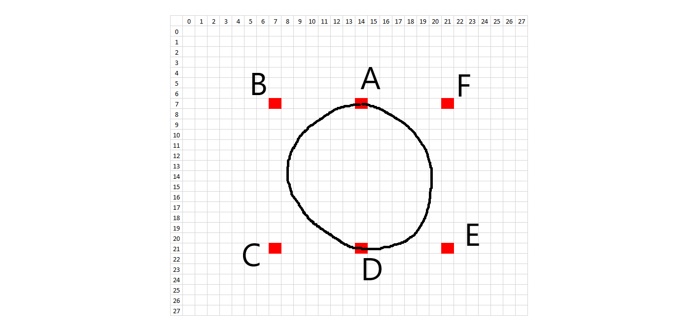
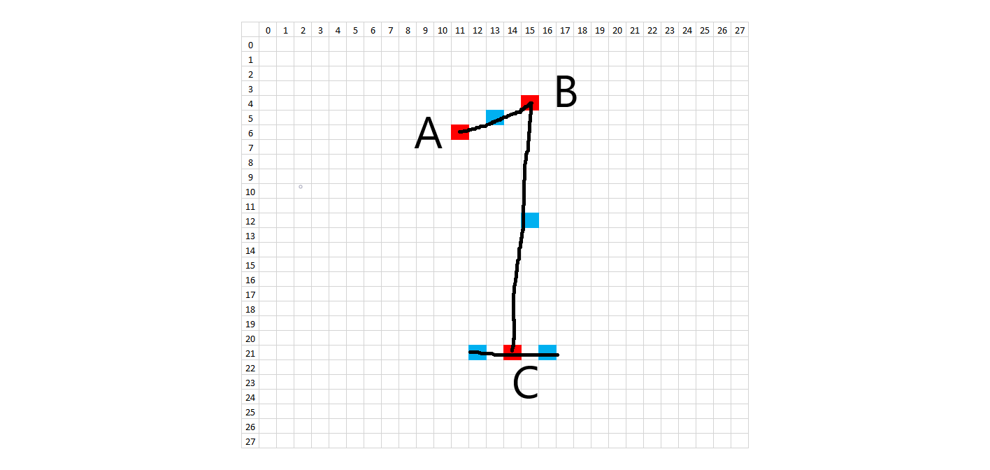
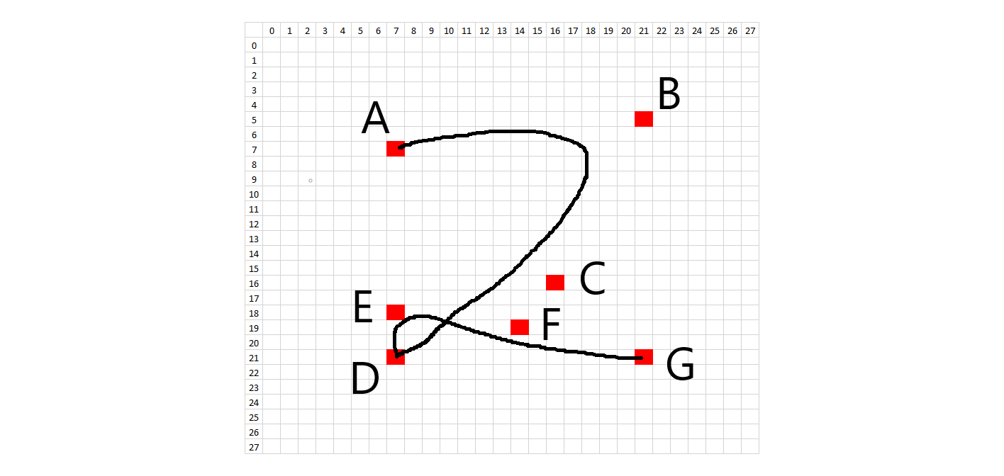
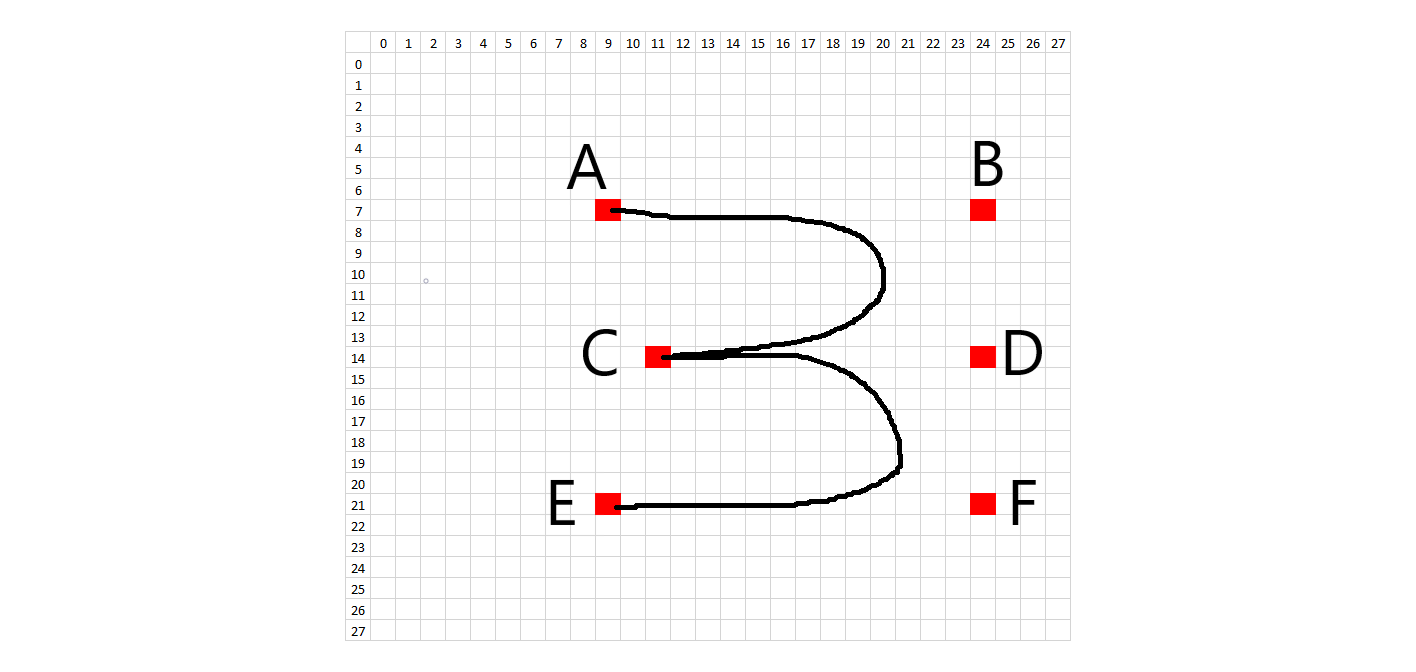
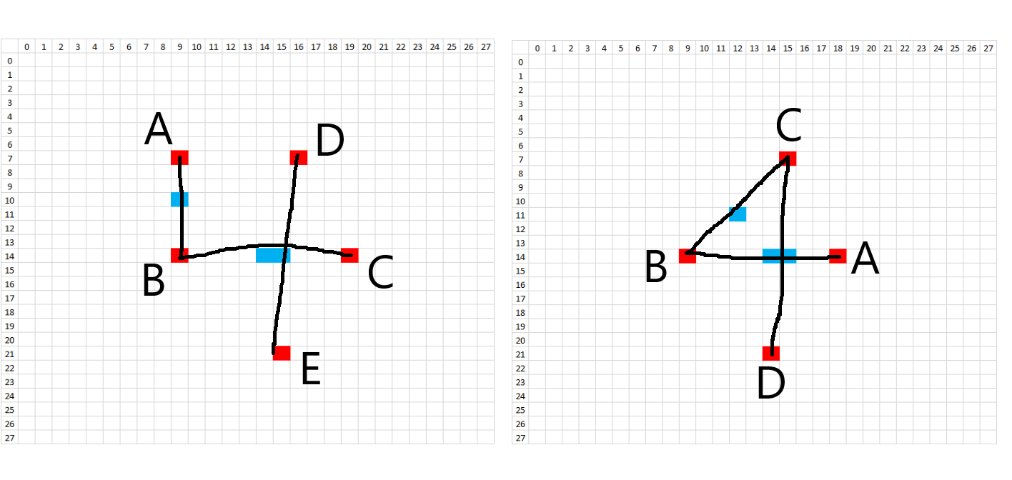
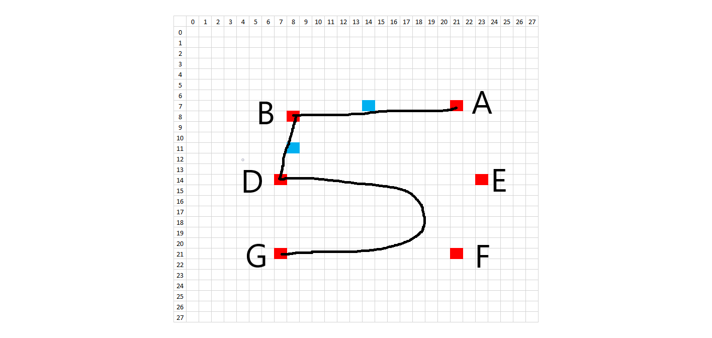
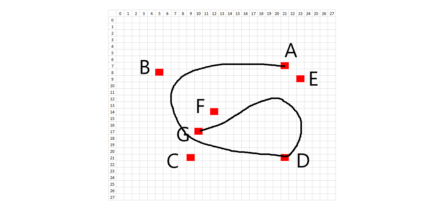
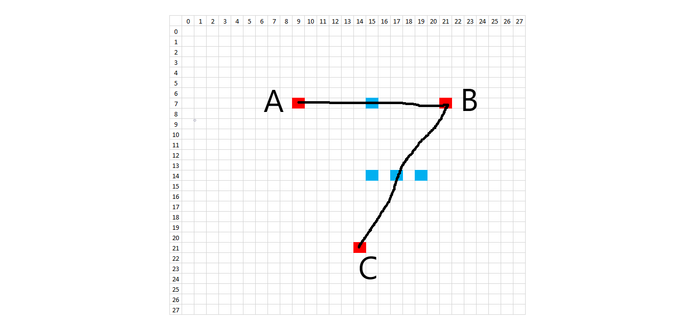
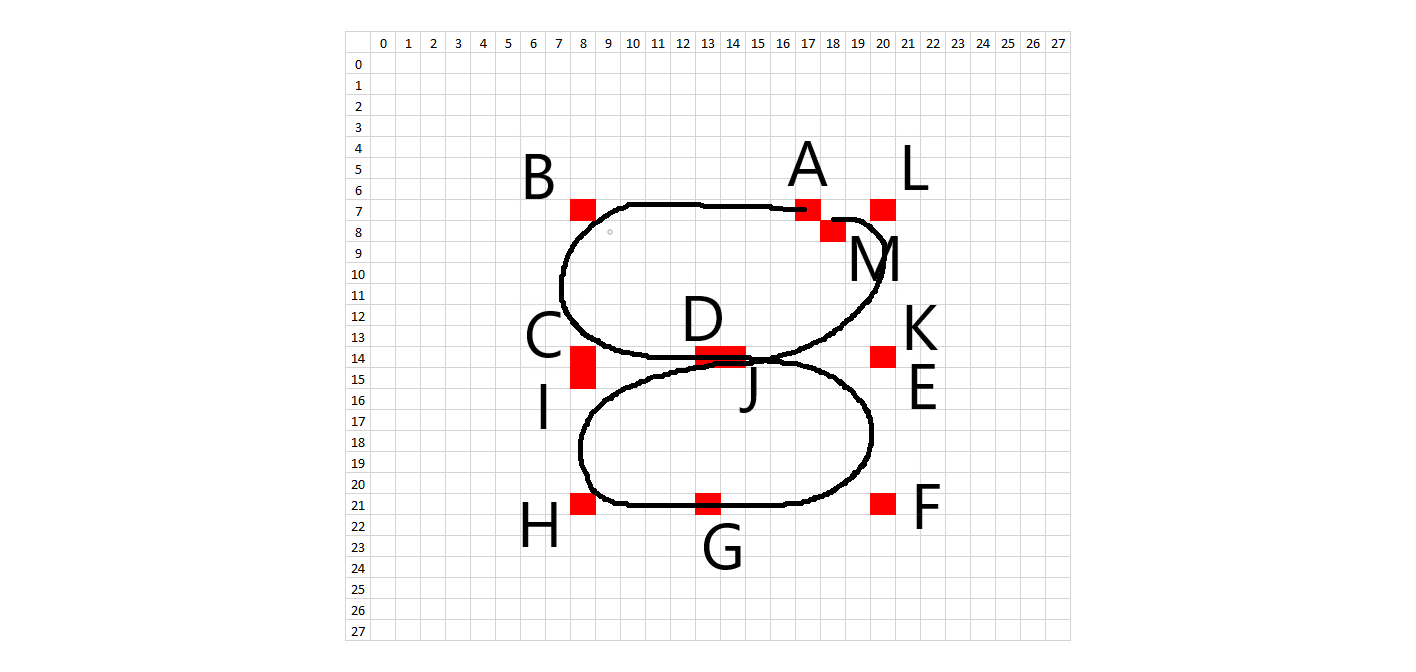
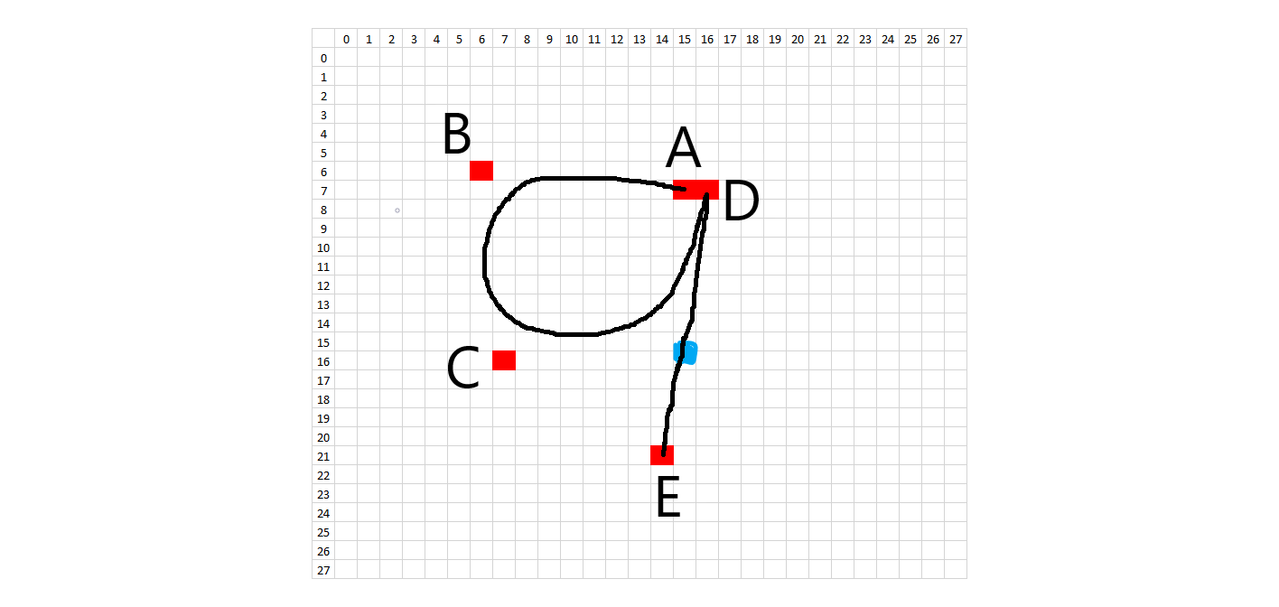
The methodology to create synthetic digits was to try to emulate the whole handwriting and digitization process as much as possible. First, I looked at the 28x28 images and picked general starting and ending points for each stroke on each digit. In order to introduce variation, each starting and ending point was allowed to vary according to random placement about that point. What would normally be a straight line in a perfectly written digit was treated as a quadratic Bezier curve in order to introduce a small amount of arc. Placement of these Bezier support points is also random, using the midpoint of the line between the two points as a starting spot. The amount of variation allowed on the control points is on a case-by-case basis. Natural curves on the digits are treated as cubic Bezier curves, where a single curve will have two endpoints and two degrees of freedom. The starting, ending, and Bezier control points are all allowed to randomly vary about an initial starting position. Each digit has a certain number of Bezier control points and the subsequent digit characteristics can be changed by modifying the Bezier control points in the code. The diagrams below show the control points.
In order to recreate the digitization process, the image is enlarged or "zoomed" to a certain size. All lines and curves are drawn on this larger canvas, to allow for greater definition. The brush stroke (pen width) also is randomly determined about some range of values, given the different brush strokes we see in the training data. In addition, the intensity of the colored pixels linearly decreases to 0 past a critical value. After all of the drawing, the images are then resized to 28x28, hopefully picking up digitization artifacts similar to the training data.
import random
from scipy.misc import imresize
from skimage.transform import resize
import cv2

def getRandomPoint(x,y,jitterRadius):
    startX = x
    startY = y
    radius = random.uniform(0,jitterRadius)
    angle = random.uniform(0,2*math.pi)
    endX = startX + radius * math.cos( angle )
    endY = startY + radius * math.sin( angle )
    return(endX,endY)

def drawLine(image, points, brushWidth):
    # if points is length 2, draw line
    # if points is length 3, draw quadratic Bezier curve
    # if points is length 4, draw cubic Bezier curve

    # make a darkness gradient so that cells a distance a way from the pen point
    # are less darkly colored.  Make so up to 1/ff brush width, the color is 1.0
    # then linearly ramp to 0
    ff = 5
    numPoints = len( points )
    totalDistance = 0
    if numPoints > 1:
        # calcululate the length of all the lines
        # dist = sqrt( ( x2 - x1 )^2 + (y2 - y1 )^2 )
        squares = [(points[i+1][0]-points[i][0])*(points[i+1][0]-points[i][0])+(points[i+1][1]-points[i][1])*(points[i+1][1]-points[i][1]) for i in range(len(points)-1)]
        totalDistance = math.sqrt( sum( squares ) )
    if numPoints == 2:
        # just a simple line
        aX   = points[0][0]
        aY   = points[0][1]
        bX   = points[1][0]
        bY   = points[1][1]
        numSteps = round( totalDistance )
        stepSize = 1/numSteps
        for t in [s/numSteps for s in range(0,numSteps+1)]:
            x = (1-t)*aX + t*bX
            y = (1-t)*aY + t*bY
            # now color brush width and every square that is within brush width/2;
            # make sure we don't paint off the end of the image
            xStart = max( round( x - brushWidth/2.0), 0 )
            xEnd = min( round( x + brushWidth/2.0 + 1), image.shape[0] )
            yStart = max( round( y - brushWidth/2.0 ), 0 )
            yEnd = min( round( y + brushWidth/2.0 + 1), image.shape[1] )
            for xcoord in range( xStart, xEnd ):
                for ycoord in range( yStart, yEnd ):
                    distToTip = math.sqrt( ( x - xcoord ) * ( x - xcoord ) + ( y - ycoord ) * ( y - ycoord ) )
                    if distToTip <= brushWidth/2:
                        if distToTip <= brushWidth/ff:
                            pixelDarkness = 1.0
                        else:
                            pctTraveled = distToTip/(brushWidth/2)
                            pixelDarkness = 1.0-pctTraveled
                        # take the max between this calc and what was already there in case there was
                        # a darker line there already
                        image[xcoord,ycoord,0] = max(image[xcoord,ycoord,0],pixelDarkness)
    elif numPoints == 3:
        aX   = points[0][0]
        aY   = points[0][1]
        bezX = points[1][0]
        bezY = points[1][1]
        bX   = points[2][0]
        bY   = points[2][1]
        # the distance between starting and ending points is totalDist.  Want to make sure all the pixels
        # in the line are colored so have to walk line slowly (stepSize) since it is not a straight line but a
        # curve. Figure the curve is at most a half circle so arc length is roughly distance * pi/2 or simply 1.5
        arcLength = totalDistance * 1.5
        numSteps = round( arcLength )
        stepSize = 1/numSteps
        for t in [s/numSteps for s in range(0,numSteps+1)]:
            x = (1-t)*(1-t)*aX + 2*(1-t)*t*bezX + t*t*bX
            y = (1-t)*(1-t)*aY + 2*(1-t)*t*bezY + t*t*bY
            # now color brush width and every square that is within brush width/2;
            # make sure we don't paint off the end of the image
            xStart = max( round( x - brushWidth/2.0), 0 )
            xEnd = min( round( x + brushWidth/2.0 + 1), image.shape[0] )
            yStart = max( round( y - brushWidth/2.0 ), 0 )
            yEnd = min( round( y + brushWidth/2.0 + 1), image.shape[1] )
            for xcoord in range( xStart, xEnd ):
                for ycoord in range( yStart, yEnd ):
                    distToTip = math.sqrt( ( x - xcoord ) * ( x - xcoord ) + ( y - ycoord ) * ( y - ycoord ) )
                    if distToTip < brushWidth/2:
                        if distToTip <= brushWidth/ff:
                            pixelDarkness = 1.0
                        else:
                            pctTraveled = distToTip/(brushWidth/2)
                            pixelDarkness = 1.0-pctTraveled
                        # take the max between this calc and what was already there in case there was
                        # a darker line there already
                        image[xcoord,ycoord,0] = max(image[xcoord,ycoord,0],pixelDarkness)
    elif numPoints == 4:
        aX    = points[0][0]
        aY    = points[0][1]
        bez1X = points[1][0]
        bez1Y = points[1][1]
        bez2X = points[2][0]
        bez2Y = points[2][1]
        cX    = points[3][0]
        cY    = points[3][1]
        # the distance between starting and ending points is totalDist.  Want to make sure all the pixels
        # in the line are colored so have to walk line slowly (stepSize) since it is not a straight line but a
        # curve. Figure the curve is more than a half circle so arc length is roughly > distance * pi/2 or simply 1.7
        arcLength = totalDistance * 1.7
        numSteps = round( arcLength )
        stepSize = 1/numSteps
        for t in [s/numSteps for s in range(0,numSteps+1)]:
            x = (1-t)*(1-t)*(1-t)*aX + 3*(1-t)*(1-t)*t*bez1X + 3*(1-t)*t*t*bez2X + t*t*t*cX
            y = (1-t)*(1-t)*(1-t)*aY + 3*(1-t)*(1-t)*t*bez1Y + 3*(1-t)*t*t*bez2Y + t*t*t*cY
            # now color brush width and every square that is within brush width/2;
            # make sure we don't paint off the end of the image
            xStart = max( round( x - brushWidth/2.0), 0 )
            xEnd = min( round( x + brushWidth/2.0 + 1), image.shape[0] )
            yStart = max( round( y - brushWidth/2.0 ), 0 )
            yEnd = min( round( y + brushWidth/2.0 + 1), image.shape[1] )
            for xcoord in range( xStart, xEnd ):
                for ycoord in range( yStart, yEnd ):
                    distToTip = math.sqrt( ( x - xcoord ) * ( x - xcoord ) + ( y - ycoord ) * ( y - ycoord ) )
                    if distToTip < brushWidth/2:
                        if distToTip <= brushWidth/ff:
                            pixelDarkness = 1.0
                        else:
                            pctTraveled = distToTip/(brushWidth/2)
                            pixelDarkness = 1.0-pctTraveled
                        # take the max between this calc and what was already there in case there was
                        # a darker line there already
                        image[xcoord,ycoord,0] = max(image[xcoord,ycoord,0],pixelDarkness)

    return image

def get0(zoomFactor,destinationRadius):
    syntheticDigit = np.zeros((28 * zoomFactor,28 * zoomFactor,1))
    brushWidth = random.uniform(2.8,5.0) * zoomFactor
    # this is for digit '0'!
    pointA = [7,14]
    pointB = [7,7]
    pointC = [21,7]
    pointD = [21,14]
    pointE = [21,21]
    pointF = [7,21]
    pointG = [7,13]

    destinationRadius *= 2

    # aX,aY are the coordinates for the top of the '0', d is the bottom; b and c are Bezier supports
    (aX,aY) = getRandomPoint(pointA[0]*zoomFactor,pointA[1]*zoomFactor,destinationRadius*zoomFactor)
    (bX,bY) = getRandomPoint(pointB[0]*zoomFactor,pointB[1]*zoomFactor,destinationRadius*zoomFactor)
    (cX,cY) = getRandomPoint(pointC[0]*zoomFactor,pointC[1]*zoomFactor,destinationRadius*zoomFactor)
    (dX,dY) = getRandomPoint(pointD[0]*zoomFactor,pointD[1]*zoomFactor,destinationRadius*zoomFactor)
    (eX,eY) = getRandomPoint(pointE[0]*zoomFactor,pointE[1]*zoomFactor,destinationRadius*zoomFactor)
    (fX,fY) = getRandomPoint(pointF[0]*zoomFactor,pointF[1]*zoomFactor,destinationRadius*zoomFactor)
    (gX,gY) = getRandomPoint(pointG[0]*zoomFactor,pointG[1]*zoomFactor,destinationRadius*zoomFactor)
    # draw left hand arc
    syntheticDigit = drawLine( syntheticDigit, [(aX,aY), (bX,bY), (cX,cY), (dX,dY)], brushWidth)
    # draw right hand arc
    syntheticDigit = drawLine( syntheticDigit, [(dX,dY), (eX,eY), (fX,fY), (gX,gY)], brushWidth)

    # now, need to downsample
    #syntheticDigit = resize(syntheticDigit,(28,28))
    #syntheticDigit = imresize(syntheticDigit,1/zoomFactor)
    syntheticDigit = cv2.resize(syntheticDigit,dsize=(28,28))
    syntheticDigit = syntheticDigit.reshape(28,28,1)

    return syntheticDigit

def get1(zoomFactor,destinationRadius):
    syntheticDigit = np.zeros((28 * zoomFactor,28 * zoomFactor,1))
    brushWidth = random.uniform(2.8,5.0) * zoomFactor
    # this is for digit '1'!
    pointA = [6,11]
    pointB = [4,15]
    pointC = [21,14]

    # bX,bY are the coordinates for the top of the '1'
    (bX,bY) = getRandomPoint(pointB[0]*zoomFactor,pointB[1]*zoomFactor,destinationRadius*zoomFactor)
    # now, randomly include that thingy that people occasionally put at the top of ones
    putThingy = bool(random.getrandbits(1))
    if putThingy:
        # get point A, get radius and angle
        (aX,aY) = getRandomPoint(pointA[0]*zoomFactor,pointA[1]*zoomFactor,destinationRadius*zoomFactor)
        # now need to calculate the Bezier point P1
        bezStartX = ( aX + bX )/2
        bezStartY = ( aY + bY )/2
        distAB = math.sqrt( ( bX-aX )*(bX-aX) + (bY-aY)*(bY-aY) )
        bezRadius = random.uniform(0,distAB/2.1)
        (bezX,bezY) = getRandomPoint(bezStartX,bezStartY,bezRadius)
        syntheticDigit = drawLine( syntheticDigit, [(aX,aY), (bezX,bezY), (bX,bY)], brushWidth)
    # okay, now draw the long line from the top of the one to the bottom
    # destination
    (cX,cY) = getRandomPoint(pointC[0]*zoomFactor,pointC[1]*zoomFactor,destinationRadius*3*zoomFactor)
    # now get Bezier point between B and C
    bezStartX = ( bX + cX )/2
    bezStartY = ( bY + cY )/2
    distBC = math.sqrt( ( cX-bX )*(cX-bX) + (cY-bY)*(cY-bY) )
    bezRadius = random.uniform(0,distBC/3.5)  # want this to be closer to the middle
    (bezX,bezY) = getRandomPoint(bezStartX,bezStartY,bezRadius)
    syntheticDigit = drawLine( syntheticDigit, [(bX,bY), (bezX,bezY), (cX,cY)], brushWidth)
    # now, figure out if we need to draw a base.  You tend to only see a base when there's a thingy.
    if putThingy:
        putBase = bool(random.getrandbits(1))
        if putBase:
            baseHalfLength = zoomFactor * 4
            (dX,dY) = getRandomPoint(cX,cY-baseHalfLength,destinationRadius*zoomFactor)
            (eX,eY) = getRandomPoint(cX,cY+baseHalfLength,destinationRadius*zoomFactor)
            syntheticDigit = drawLine( syntheticDigit, [(dX,dY), (cX,cY), (eX,eY)], brushWidth)

    # now, need to downsample
    #syntheticDigit = resize(syntheticDigit,(28,28))
    #syntheticDigit = imresize(syntheticDigit,1/zoomFactor)
    syntheticDigit = cv2.resize(syntheticDigit,dsize=(28,28))
    syntheticDigit = syntheticDigit.reshape(28,28,1)

    return syntheticDigit

def get2(zoomFactor,destinationRadius):
    syntheticDigit = np.zeros((28 * zoomFactor,28 * zoomFactor,1))
    brushWidth = random.uniform(2.8,5.0) * zoomFactor
    # this is for digit '2'!
    pointA = [7,7]
    pointB = [5,21]
    pointC = [16,16]
    pointD = [21,7]
    pointE = [18,7]
    pointF = [19,14]
    pointG = [21,21]

    destinationRadius *= 2

    # aX,aY are the coordinates for the top of the '0', d is the bottom; b and c are Bezier supports
    (aX,aY) = getRandomPoint(pointA[0]*zoomFactor,pointA[1]*zoomFactor,destinationRadius*zoomFactor)
    (bX,bY) = getRandomPoint(pointB[0]*zoomFactor,pointB[1]*zoomFactor,destinationRadius*zoomFactor)
    (cX,cY) = getRandomPoint(pointC[0]*zoomFactor,pointC[1]*zoomFactor,destinationRadius*zoomFactor)
    (dX,dY) = getRandomPoint(pointD[0]*zoomFactor,pointD[1]*zoomFactor,destinationRadius*zoomFactor)
    (eX,eY) = getRandomPoint(pointE[0]*zoomFactor,pointE[1]*zoomFactor,destinationRadius*zoomFactor)
    (fX,fY) = getRandomPoint(pointF[0]*zoomFactor,pointF[1]*zoomFactor,destinationRadius*zoomFactor)
    (gX,gY) = getRandomPoint(pointG[0]*zoomFactor,pointG[1]*zoomFactor,destinationRadius*zoomFactor)
    # draw left hand arc
    syntheticDigit = drawLine( syntheticDigit, [(aX,aY), (bX,bY), (cX,cY), (dX,dY)], brushWidth)
    # draw right hand arc
    syntheticDigit = drawLine( syntheticDigit, [(dX,dY), (eX,eY), (fX,fY), (gX,gY)], brushWidth)

    # now, need to downsample
    #syntheticDigit = resize(syntheticDigit,(28,28))
    #syntheticDigit = imresize(syntheticDigit,1/zoomFactor)
    syntheticDigit = cv2.resize(syntheticDigit,dsize=(28,28))
    syntheticDigit = syntheticDigit.reshape(28,28,1)

    return syntheticDigit

def get3(zoomFactor,destinationRadius):
    syntheticDigit = np.zeros((28 * zoomFactor,28 * zoomFactor,1))
    brushWidth = random.uniform(2.8,5.0) * zoomFactor
    # this is for digit '2'!
    pointA = [7,9]
    pointB = [7,24]
    pointC = [14,24]
    pointD = [14,11]
    pointE = [14,24]
    pointF = [21,24]
    pointG = [21,9]

    destinationRadius *= 2

    # aX,aY are the coordinates for the top of the '0', d is the bottom; b and c are Bezier supports
    (aX,aY) = getRandomPoint(pointA[0]*zoomFactor,pointA[1]*zoomFactor,destinationRadius*zoomFactor)
    (bX,bY) = getRandomPoint(pointB[0]*zoomFactor,pointB[1]*zoomFactor,destinationRadius*zoomFactor)
    (cX,cY) = getRandomPoint(pointC[0]*zoomFactor,pointC[1]*zoomFactor,destinationRadius*zoomFactor)
    (dX,dY) = getRandomPoint(pointD[0]*zoomFactor,pointD[1]*zoomFactor,destinationRadius*zoomFactor)
    (eX,eY) = getRandomPoint(pointE[0]*zoomFactor,pointE[1]*zoomFactor,destinationRadius*zoomFactor)
    (fX,fY) = getRandomPoint(pointF[0]*zoomFactor,pointF[1]*zoomFactor,destinationRadius*zoomFactor)
    (gX,gY) = getRandomPoint(pointG[0]*zoomFactor,pointG[1]*zoomFactor,destinationRadius*zoomFactor)
    # draw left hand arc
    syntheticDigit = drawLine( syntheticDigit, [(aX,aY), (bX,bY), (cX,cY), (dX,dY)], brushWidth)
    # draw right hand arc
    syntheticDigit = drawLine( syntheticDigit, [(dX,dY), (eX,eY), (fX,fY), (gX,gY)], brushWidth)

    # now, need to downsample
    #syntheticDigit = resize(syntheticDigit,(28,28))
    #syntheticDigit = imresize(syntheticDigit,1/zoomFactor)
    syntheticDigit = cv2.resize(syntheticDigit,dsize=(28,28))
    syntheticDigit = syntheticDigit.reshape(28,28,1)

    return syntheticDigit

def get4(zoomFactor,destinationRadius):
    # there are two main ways to make a number 4: one with the pen leaving the paper once
    # (like a checkmark and a cross through it).  The other way is in one motion, with the
    # pen never leaving the paper.  I figure the 2nd way of doing it isn't as prevalent, so
    # make the probability of that one happening something like 15%.  Hey, I just noticed
    # that this four -> 4 <- is of the 2nd variety!
    probabilityOfWeird4 = 0.15
    pickANumber = random.random()  # between 0 and 1
    if pickANumber > probabilityOfWeird4:
        return get4a(zoomFactor,destinationRadius)
    else:
        return get4b(zoomFactor,destinationRadius)

def get4a(zoomFactor,destinationRadius):
    syntheticDigit = np.zeros((28 * zoomFactor,28 * zoomFactor,1))
    brushWidth = random.uniform(2.8,5.0) * zoomFactor
    # this is for digit '4', the common one
    pointA = [7,10]
    pointB = [14,9]
    pointC = [14,19]
    pointD = [7,16]
    pointE = [21,15]

    (aX,aY) = getRandomPoint(pointA[0]*zoomFactor,pointA[1]*zoomFactor,destinationRadius*zoomFactor)
    (bX,bY) = getRandomPoint(pointB[0]*zoomFactor,pointB[1]*zoomFactor,destinationRadius*zoomFactor)
    (cX,cY) = getRandomPoint(pointC[0]*zoomFactor,pointC[1]*zoomFactor,destinationRadius*zoomFactor)
    (dX,dY) = getRandomPoint(pointD[0]*zoomFactor,pointD[1]*zoomFactor,destinationRadius*zoomFactor)
    (eX,eY) = getRandomPoint(pointE[0]*zoomFactor,pointE[1]*zoomFactor,destinationRadius*zoomFactor)

    # get Bezier support between A and B.  Don't want this to be a big arc though because generally
    # that first line of a 4 is pretty straight.  People don't start messing up until the 2nd line
    bezStartX = ( aX + bX )/2
    bezStartY = ( aY + bY )/2
    distAB = math.sqrt( ( bX-aX )*(bX-aX) + (bY-aY)*(bY-aY) )
    bezRadius = random.uniform(0,distAB/4)
    (bezX,bezY) = getRandomPoint(bezStartX,bezStartY,bezRadius)
    syntheticDigit = drawLine( syntheticDigit, [(aX,aY), (bezX,bezY), (bX,bY)], brushWidth)
    # okay, now draw the 2nd line from left to right
    # first get Bezier point between B and C
    bezStartX = ( bX + cX )/2
    bezStartY = ( bY + cY )/2
    distBC = math.sqrt( ( cX-bX )*(cX-bX) + (cY-bY)*(cY-bY) )
    bezRadius = random.uniform(0,distBC/2.1)  # this can have a little bit of arc to it
    (bezX,bezY) = getRandomPoint(bezStartX,bezStartY,bezRadius)
    syntheticDigit = drawLine( syntheticDigit, [(bX,bY), (bezX,bezY), (cX,cY)], brushWidth)
    # now, draw the big line down the middle
    # first get Bezier support
    bezStartX = ( dX + eX )/2
    bezStartY = ( dY + eY )/2
    distDE = math.sqrt( ( eX-dX )*(eX-dX) + (eY-dY)*(eY-dY) )
    bezRadius = random.uniform(0,distDE/4)  # this can have a little bit of arc to it
    (bezX,bezY) = getRandomPoint(bezStartX,bezStartY,bezRadius)
    syntheticDigit = drawLine( syntheticDigit, [(dX,dY), (bezX,bezY), (eX,eY)], brushWidth)

    # now, need to downsample
    #syntheticDigit = resize(syntheticDigit,(28,28))
    #syntheticDigit = imresize(syntheticDigit,1/zoomFactor)
    syntheticDigit = cv2.resize(syntheticDigit,dsize=(28,28))
    syntheticDigit = syntheticDigit.reshape(28,28,1)

    return syntheticDigit

def get4b(zoomFactor,destinationRadius):
    syntheticDigit = np.zeros((28 * zoomFactor,28 * zoomFactor,1))
    brushWidth = random.uniform(2.8,5.0) * zoomFactor
    # this is for digit '4', the secondary one.  Since I don't write these, I'm not sure
    # which end to start and while it seems arbitrary, I want to follow what humans do as
    # much as possible.  Guess we'll start at the right hand side and work towards the bottom
    pointA = [14,18]
    pointB = [14,9]
    pointC = [7,15]
    pointD = [21,14]

    (aX,aY) = getRandomPoint(pointA[0]*zoomFactor,pointA[1]*zoomFactor,destinationRadius*zoomFactor)
    (bX,bY) = getRandomPoint(pointB[0]*zoomFactor,pointB[1]*zoomFactor,destinationRadius*zoomFactor)
    (cX,cY) = getRandomPoint(pointC[0]*zoomFactor,pointC[1]*zoomFactor,destinationRadius*zoomFactor)
    (dX,dY) = getRandomPoint(pointD[0]*zoomFactor,pointD[1]*zoomFactor,destinationRadius*zoomFactor)

    # get Bezier support between A and B.  Don't want this to be a big arc though because generally
    # that first line of a 4 is pretty straight.  People don't start messing up until the 2nd line
    bezStartX = ( aX + bX )/2
    bezStartY = ( aY + bY )/2
    distAB = math.sqrt( ( bX-aX )*(bX-aX) + (bY-aY)*(bY-aY) )
    bezRadius = random.uniform(0,distAB/4)
    (bezX,bezY) = getRandomPoint(bezStartX,bezStartY,bezRadius)
    syntheticDigit = drawLine( syntheticDigit, [(aX,aY), (bezX,bezY), (bX,bY)], brushWidth)
    # okay, now draw the 2nd line from left to right
    # first get Bezier point between B and C
    bezStartX = ( bX + cX )/2
    bezStartY = ( bY + cY )/2
    distBC = math.sqrt( ( cX-bX )*(cX-bX) + (cY-bY)*(cY-bY) )
    bezRadius = random.uniform(0,distBC/3.1)  # this can have a little bit of arc to it
    (bezX,bezY) = getRandomPoint(bezStartX,bezStartY,bezRadius)
    syntheticDigit = drawLine( syntheticDigit, [(bX,bY), (bezX,bezY), (cX,cY)], brushWidth)
    # now, draw the big line down the middle
    # first get Bezier support
    bezStartX = ( cX + dX )/2
    bezStartY = ( cY + dY )/2
    distCD = math.sqrt( ( dX-cX )*(dX-cX) + (dY-cY)*(dY-cY) )
    bezRadius = random.uniform(0,distCD/4)  # this can have a little bit of arc to it
    (bezX,bezY) = getRandomPoint(bezStartX,bezStartY,bezRadius)
    syntheticDigit = drawLine( syntheticDigit, [(cX,cY), (bezX,bezY), (dX,dY)], brushWidth)

    # now, need to downsample
    #syntheticDigit = resize(syntheticDigit,(28,28))
    #syntheticDigit = imresize(syntheticDigit,1/zoomFactor)
    syntheticDigit = cv2.resize(syntheticDigit,dsize=(28,28))
    syntheticDigit = syntheticDigit.reshape(28,28,1)

    return syntheticDigit

def get5(zoomFactor,destinationRadius):
    syntheticDigit = np.zeros((28 * zoomFactor,28 * zoomFactor,1))
    brushWidth = random.uniform(2.8,5.0) * zoomFactor
    # this is for digit '4', the common one
    pointA = [8,8]
    pointB = [7,21]
    pointC = [8,8]  # not used
    pointD = [14,7]
    pointE = [14,23]
    pointF = [21,21]
    pointG = [21,7]

    (aX,aY) = getRandomPoint(pointA[0]*zoomFactor,pointA[1]*zoomFactor,destinationRadius*zoomFactor)
    (bX,bY) = getRandomPoint(pointB[0]*zoomFactor,pointB[1]*zoomFactor,destinationRadius*zoomFactor)
    (cX,cY) = getRandomPoint(aX,aY,destinationRadius*0.5*zoomFactor)  # base off of aX,aY
    (dX,dY) = getRandomPoint(pointD[0]*zoomFactor,pointD[1]*zoomFactor,2*destinationRadius*zoomFactor)
    (eX,eY) = getRandomPoint(pointE[0]*zoomFactor,pointE[1]*zoomFactor,destinationRadius*zoomFactor)
    (fX,fY) = getRandomPoint(pointF[0]*zoomFactor,pointF[1]*zoomFactor,destinationRadius*zoomFactor)
    (gX,gY) = getRandomPoint(pointG[0]*zoomFactor,pointG[1]*zoomFactor,destinationRadius*zoomFactor)

    # get Bezier support between A and B.  Don't want this to be a big arc though because generally
    # that first line of a 5 is pretty straight.
    bezStartX = ( aX + bX )/2
    bezStartY = ( aY + bY )/2
    distAB = math.sqrt( ( bX-aX )*(bX-aX) + (bY-aY)*(bY-aY) )
    bezRadius = random.uniform(0,distAB/4)
    (bezX,bezY) = getRandomPoint(bezStartX,bezStartY,bezRadius)
    syntheticDigit = drawLine( syntheticDigit, [(aX,aY), (bezX,bezY), (bX,bY)], brushWidth)
    # okay, now draw the 2nd line from left to right
    # first get Bezier point between C and D
    bezStartX = ( cX + dX )/2
    bezStartY = ( cY + dY )/2
    distCD = math.sqrt( ( dX-cX )*(dX-cX) + (dY-cY)*(dY-cY) )
    bezRadius = random.uniform(0,distCD/3.1)  # this can have a little bit of arc to it
    (bezX,bezY) = getRandomPoint(bezStartX,bezStartY,bezRadius)
    syntheticDigit = drawLine( syntheticDigit, [(cX,cY), (bezX,bezY), (dX,dY)], brushWidth)
    # now, draw the big arc of the 5 w/ cubic Bezier curve
    # first get Bezier support
    syntheticDigit = drawLine( syntheticDigit, [(dX,dY), (eX,eY), (fX,fY), (gX,gY)], brushWidth)

    # now, need to downsample
    #syntheticDigit = resize(syntheticDigit,(28,28))
    #syntheticDigit = imresize(syntheticDigit,1/zoomFactor)
    syntheticDigit = cv2.resize(syntheticDigit,dsize=(28,28))
    syntheticDigit = syntheticDigit.reshape(28,28,1)

    return syntheticDigit

def get6(zoomFactor,destinationRadius):
    # not super pleased by the lack of diversity of the loops that I'm seeing
    # would like to make a model which has an oblong loop aligned with initial large sweeping arc
    syntheticDigit = np.zeros((28 * zoomFactor,28 * zoomFactor,1))
    brushWidth = random.uniform(2.8,5.0) * zoomFactor
    # this is for digit '6'
    pointA = [7,21]
    pointB = [8,5]
    pointC = [21,9]
    pointD = [21,21]
    pointE = [9,23]
    pointF = [14,12]
    pointG = [17,10]

    (aX,aY) = getRandomPoint(pointA[0]*zoomFactor,pointA[1]*zoomFactor,destinationRadius*zoomFactor)
    (bX,bY) = getRandomPoint(pointB[0]*zoomFactor,pointB[1]*zoomFactor,destinationRadius*zoomFactor)
    (cX,cY) = getRandomPoint(pointC[0]*zoomFactor,pointC[1]*zoomFactor,destinationRadius*zoomFactor)
    (dX,dY) = getRandomPoint(pointD[0]*zoomFactor,pointD[1]*zoomFactor,destinationRadius*zoomFactor)
    (eX,eY) = getRandomPoint(pointE[0]*zoomFactor,pointE[1]*zoomFactor,destinationRadius*zoomFactor)
    (fX,fY) = getRandomPoint(pointF[0]*zoomFactor,pointF[1]*zoomFactor,destinationRadius*zoomFactor)
    (gX,gY) = getRandomPoint(pointG[0]*zoomFactor,pointG[1]*zoomFactor,destinationRadius*zoomFactor)

    syntheticDigit = drawLine( syntheticDigit, [(aX,aY), (bX,bY), (cX,cY), (dX,dY)], brushWidth)
    syntheticDigit = drawLine( syntheticDigit, [(dX,dY), (eX,eY), (fX,fY), (gX,gY)], brushWidth)

    # now, need to downsample
    #syntheticDigit = resize(syntheticDigit,(28,28))
    #syntheticDigit = imresize(syntheticDigit,1/zoomFactor)
    syntheticDigit = cv2.resize(syntheticDigit,dsize=(28,28))
    syntheticDigit = syntheticDigit.reshape(28,28,1)

    return syntheticDigit

def get7(zoomFactor,destinationRadius):
    syntheticDigit = np.zeros((28 * zoomFactor,28 * zoomFactor,1))
    brushWidth = random.uniform(3.2,5.0) * zoomFactor
    # this is for digit '7'!
    pointA = [7,9]
    pointB = [7,21]
    pointC = [21,14]

    (aX,aY) = getRandomPoint(pointA[0]*zoomFactor,pointA[1]*zoomFactor,destinationRadius*zoomFactor)
    (bX,bY) = getRandomPoint(pointB[0]*zoomFactor,pointB[1]*zoomFactor,destinationRadius*zoomFactor)
    (cX,cY) = getRandomPoint(pointC[0]*zoomFactor,pointC[1]*zoomFactor,destinationRadius*zoomFactor)

    # now, randomly include that thingy that people occasionally hang off the front of their sevens.  I'm guessing
    # it shows up 15% of the time.
    putThingy = False
    probabilityOfThingy = 0.15
    pickANumber = random.random()  # between 0 and 1
    if pickANumber < probabilityOfThingy:
        putThingy = True
    if putThingy:
        thingyLength = 1.6
        thingyX = aX + thingyLength * zoomFactor
        thingyY = aY
        syntheticDigit = drawLine( syntheticDigit, [(aX,aY), (thingyX,thingyY)], brushWidth)

    # get Bezier support between A and B (top line of 7)
    bezStartX = ( aX + bX )/2
    bezStartY = ( aY + bY )/2
    distAB = math.sqrt( ( bX-aX )*(bX-aX) + (bY-aY)*(bY-aY) )
    bezRadius = random.uniform(0,distAB/3)
    (bezX,bezY) = getRandomPoint(bezStartX,bezStartY,bezRadius)
    syntheticDigit = drawLine( syntheticDigit, [(aX,aY), (bezX,bezY), (bX,bY)], brushWidth)

     # okay, now draw the line to the bottom
    # first get Bezier point between B and C
    bezStartX = ( bX + cX )/2
    bezStartY = ( bY + cY )/2
    distBC = math.sqrt( ( cX-bX )*(cX-bX) + (cY-bY)*(cY-bY) )
    bezRadius = random.uniform(0,distBC/2.1)  # this can have a lot of arc to it
    (bezX,bezY) = getRandomPoint(bezStartX,bezStartY,bezRadius)
    syntheticDigit = drawLine( syntheticDigit, [(bX,bY), (bezX,bezY), (cX,cY)], brushWidth)

    # now, randomly include that dash that people occasionally put through their sevens.  I'm guessing
    # it shows up 10% of the time.
    putDash = False
    probabilityOfDash = 0.10
    pickANumber = random.random()  # between 0 and 1
    if pickANumber < probabilityOfDash:
        putDash = True
    if putDash:
        # now need to calculate the Bezier point P1
        bezX = ( bX + cX )/2
        bezY = ( bY + cY )/2
        distBC = math.sqrt( ( cX-bX )*(cX-bX) + (cY-bY)*(cY-bY) )
        bezRadius = random.uniform(0,distBC/7.1)
        dashLength = 5
        (dX,dY) = getRandomPoint(bezX,bezY - (dashLength/2)*zoomFactor,bezRadius)
        (eX,eY) = getRandomPoint(bezX,bezY + (dashLength/2)*zoomFactor,bezRadius)
        syntheticDigit = drawLine( syntheticDigit, [(dX,dY), (bezX,bezY), (eX,eY)], brushWidth)

    # now, need to downsample
    #syntheticDigit = resize(syntheticDigit,(28,28))
    #syntheticDigit = imresize(syntheticDigit,1/zoomFactor)
    syntheticDigit = cv2.resize(syntheticDigit,dsize=(28,28))
    syntheticDigit = syntheticDigit.reshape(28,28,1)

    return syntheticDigit

def get8(zoomFactor,destinationRadius):
    destinationRadius *= 2
    syntheticDigit = np.zeros((28 * zoomFactor,28 * zoomFactor,1))
    brushWidth = random.uniform(3.2,5.0) * zoomFactor
    # this is for digit '8'
    pointA = [7,17]
    pointB = [7,8]
    pointC = [14,8]
    pointD = [14,13]
    pointE = [14,20]
    pointF = [21,20]
    pointG = [21,13]
    pointH = [21,8]
    pointI = [14,8]
    pointJ = [14,14]
    pointK = [14,20]
    pointL = [7,20]
    pointM = [7,17]

    (aX,aY) = getRandomPoint(pointA[0]*zoomFactor,pointA[1]*zoomFactor,destinationRadius*zoomFactor)
    (bX,bY) = getRandomPoint(pointB[0]*zoomFactor,pointB[1]*zoomFactor,destinationRadius*zoomFactor)
    (cX,cY) = getRandomPoint(pointC[0]*zoomFactor,pointC[1]*zoomFactor,destinationRadius*zoomFactor)
    (dX,dY) = getRandomPoint(pointD[0]*zoomFactor,pointD[1]*zoomFactor,destinationRadius*zoomFactor)
    (eX,eY) = getRandomPoint(pointE[0]*zoomFactor,pointE[1]*zoomFactor,destinationRadius*zoomFactor)
    (fX,fY) = getRandomPoint(pointF[0]*zoomFactor,pointF[1]*zoomFactor,destinationRadius*zoomFactor)
    (gX,gY) = getRandomPoint(pointG[0]*zoomFactor,pointG[1]*zoomFactor,destinationRadius*0.5*zoomFactor)
    (hX,hY) = getRandomPoint(pointH[0]*zoomFactor,pointH[1]*zoomFactor,destinationRadius*zoomFactor)
    (iX,iY) = getRandomPoint(pointI[0]*zoomFactor,pointI[1]*zoomFactor,destinationRadius*zoomFactor)
    (jX,jY) = getRandomPoint(pointJ[0]*zoomFactor,pointJ[1]*zoomFactor,destinationRadius*zoomFactor)
    (kX,kY) = getRandomPoint(pointK[0]*zoomFactor,pointK[1]*zoomFactor,destinationRadius*zoomFactor)
    (lX,lY) = getRandomPoint(pointL[0]*zoomFactor,pointL[1]*zoomFactor,destinationRadius*zoomFactor)
    (mX,mY) = getRandomPoint(pointM[0]*zoomFactor,pointM[1]*zoomFactor,destinationRadius*zoomFactor)

    syntheticDigit = drawLine( syntheticDigit, [(aX,aY), (bX,bY), (cX,cY), (dX,dY)], brushWidth)
    syntheticDigit = drawLine( syntheticDigit, [(dX,dY), (eX,eY), (fX,fY), (gX,gY)], brushWidth)
    syntheticDigit = drawLine( syntheticDigit, [(gX,gY), (hX,hY), (iX,iY), (jX,jY)], brushWidth)
    syntheticDigit = drawLine( syntheticDigit, [(jX,jY), (kX,kY), (lX,lY), (mX,mY)], brushWidth)

    # now, need to downsample
    #syntheticDigit = resize(syntheticDigit,(28,28))
    #syntheticDigit = imresize(syntheticDigit,1/zoomFactor)
    syntheticDigit = cv2.resize(syntheticDigit,dsize=(28,28))
    syntheticDigit = syntheticDigit.reshape(28,28,1)

    return syntheticDigit

def get9(zoomFactor,destinationRadius):
    syntheticDigit = np.zeros((28 * zoomFactor,28 * zoomFactor,1))
    brushWidth = random.uniform(3.2,5.0) * zoomFactor
    # this is for digit '9'!
    pointA = [7,15]
    pointB = [6,3]
    pointC = [21,11]
    pointD = [7,16]
    pointE = [21,14]

    (aX,aY) = getRandomPoint(pointA[0]*zoomFactor,pointA[1]*zoomFactor,destinationRadius*zoomFactor)
    (bX,bY) = getRandomPoint(pointB[0]*zoomFactor,pointB[1]*zoomFactor,destinationRadius*zoomFactor)
    (cX,cY) = getRandomPoint(pointC[0]*zoomFactor,pointC[1]*zoomFactor,destinationRadius*zoomFactor)
    (dX,dY) = getRandomPoint(pointD[0]*zoomFactor,pointD[1]*zoomFactor,destinationRadius*zoomFactor)
    (eX,eY) = getRandomPoint(pointE[0]*zoomFactor,pointE[1]*zoomFactor,destinationRadius*zoomFactor)

    # start with loop
    syntheticDigit = drawLine( syntheticDigit, [(aX,aY), (bX,bY), (cX,cY), (dX,dY)], brushWidth)

    # get Bezier support between D and E (vertical part of the 9)
    bezStartX = ( dX + eX )/2
    bezStartY = ( dY + eY )/2
    distDE = math.sqrt( ( eX-dX )*(eX-dX) + (eY-dY)*(eY-dY) )
    bezRadius = random.uniform(0,distDE/3)
    (bezX,bezY) = getRandomPoint(bezStartX,bezStartY,bezRadius)
    syntheticDigit = drawLine( syntheticDigit, [(dX,dY), (bezX,bezY), (eX,eY)], brushWidth)

    # now, need to downsample
    #syntheticDigit = resize(syntheticDigit,(28,28))
    #syntheticDigit = imresize(syntheticDigit,1/zoomFactor)
    syntheticDigit = cv2.resize(syntheticDigit,dsize=(28,28))
    syntheticDigit = syntheticDigit.reshape(28,28,1)

    return syntheticDigit

def getDigit(number,zoomFactor,radius):
    if number == 0:
        return get0(zoomFactor,radius)
    elif number == 1:
        return get1(zoomFactor,radius)
    elif number == 2:
        return get2(zoomFactor,radius)
    elif number == 3:
        return get3(zoomFactor,radius)
    elif number == 4:
        return get4(zoomFactor,radius)
    elif number == 5:
        return get5(zoomFactor,radius)
    elif number == 6:
        return get6(zoomFactor,radius)
    elif number == 7:
        return get7(zoomFactor,radius)
    elif number == 8:
        return get8(zoomFactor,radius)
    elif number == 9:
        return get9(zoomFactor,radius)
Generating "Bad" Digits
The idea behind the synthetic digit generator is to create a set of poorly written digits that could be pooled with the training data in order to make the network more robust to the (presumably) rare outlier cases. With that in mind, synthetic data could be generated and tested against a candidate model. The cases that fail could be collected and added to the training data and the whole set could be used to retrain the network. Ideally, this would happen in generator code so that "bad" cases could be augmented to the training data on the fly.
The digit generation code is not fast. But the framework could prove useful should it be necessary to generate more poorly written digit data. The code below shows the results of this current model against the synthetic digits with an increasing amount of jitter about each Bezier control point. The model definitely starts breaking down at higher jitter levels, especially the 8s - so there may be a better way of modeling that digit.
Note: I did not do any data augmentation with synthetic digits as my training time is already too slow to allow any sort of real experimentation. I hope to get a graphics card and revisit this problem.
zoomFactor = 10
jitterRadii = [0, 0.5, 1, 2, 3, 4, 5]

numDigitsToSample = 100   # was 100, reduced for Kaggle kernel

truth = []
call = []
maxCols = 5

for jitterRadius in jitterRadii:
    for i in range(10):
        numRows = 2
        numCols = maxCols
        numExamples = numRows * numCols
        fig, ax = plt.subplots(numRows,numCols,sharex=True,sharey=True,figsize=(14,3 * numRows))
        fig.suptitle( "Synthetic " + str(i) + " with jitter " + str(jitterRadius), fontsize=18)
        for j in range(numDigitsToSample):
            syntheticDigit = getDigit(i,zoomFactor,jitterRadius)
            d = syntheticDigit.reshape(-1,28,28,1)
            pred = model.predict(d)
            maxProb = pred.max(axis=1)[0]
            truthProb = pred[0][i]
            predCall = np.argmax(pred,axis=1)[0]
            call.append( predCall )
            truth.append( i )
            if j < numExamples:
                row = math.floor( j / maxCols )
                col = j % maxCols
                plotTitle = "Predicted: {:1d} ({:0.2f})\nTruth: {:1d} ({:0.2f})".format(predCall,maxProb,i,truthProb)
                if ax.ndim == 1:
                    ax[col].imshow(syntheticDigit[:,:,0])
                    ax[col].set_title(plotTitle)
                else:
                    ax[row,col].imshow(syntheticDigit[:,:,0])
                    ax[row,col].set_title(plotTitle)

    confusion_mat = confusion_matrix(truth, call)
    df_cm = pd.DataFrame(confusion_mat, index = [i for i in range(0,10)], columns = [i for i in range(0,10)])
    plt.figure(figsize = (6,5))
    conf_mat = sns.heatmap(df_cm, annot=True, cmap='Blues', fmt='g', cbar = False)
    conf_mat.set(xlabel='Predictions', ylabel='Truth')
    ax = plt.axes()
    ax.set_title('Synthetic Data with jitter ' + str(jitterRadius))
    truth = []
    call = []


Kaggle Results
# predict the test set
test_pred = model.predict(test)
# select the indix with the maximum probability
test_calls = np.argmax(test_pred,axis = 1)
results = pd.Series(test_calls,name="Label")

dataFrame = pd.concat([pd.Series(range(1,testRows.shape[0]+1),name = "ImageId"),results],axis = 1)
dataFrame.to_csv("MNIST_CNN.csv",index=False)
The Kaggle score is 0.99085. Not the best Kaggle score ever, but not too bad. Most of all, it's encouraging to see the test score be reflective of the validation score of 0.99. That means we really could try different things and likely trust that the validation score is representative of real world (test) data.
I hope this notebook was useful. Thanks for reading along.